Deployment of virtual sensors

Along urban routes

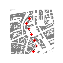
The objective here is to learn how to sample a linear path using the t4gpd.morph.STPointsDensifier class. Its constructor has 5 arguments: the first one corresponds to the name of the GeoDataFrame to sample, the second one corresponds to the value of the sampling step, the last three are optional.

STPointsDensifier(gdf, distance, pathidFieldname=None, adjustableDist=True, removeDuplicate=True)

from t4gpd.demos.GeoDataFrameDemos import GeoDataFrameDemos
from t4gpd.morph.STPointsDensifier import STPointsDensifier

pathways = GeoDataFrameDemos.districtRoyaleInNantesPaths()
pathways = pathways[ pathways.gid == 2 ]

sensors = STPointsDensifier(pathways, distance=45.0,
    pathidFieldname=None, adjustableDist=True, 
    removeDuplicate=False).run()

To map it via matplotlib, proceed as follows:

import matplotlib.pyplot as plt

_, basemap = plt.subplots(figsize=(0.25*8.26, 0.25*8.26))
buildings.plot(ax=basemap, color='grey', edgecolor='white', linewidth=0.5)
pathways.plot(ax=basemap, color='black', linewidth=0.5)
sensors.plot(ax=basemap, color='red', marker='P')
plt.axis('off')
plt.savefig('img/demo4.png')

Note: This mapping presupposes that you have already loaded the building footprints.

On the vertices of a grid

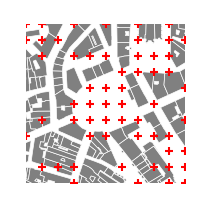
Gridding is a well-known spatial sampling technique. To grid a study space, t4gpd provides the geoprocessing name t4gpd.morph.STGrid.

STGrid(gdf, dx, dy=None, indoor=None, intoPoint=True, encode=True)

from t4gpd.demos.GeoDataFrameDemos import GeoDataFrameDemos
from t4gpd.morph.STGrid import STGrid

buildings = GeoDataFrameDemos.districtRoyaleInNantesBuildings()

sensors = STGrid(buildings, dx=20, dy=None, indoor=False, intoPoint=True).run()

To map it via matplotlib, proceed as follows:

import matplotlib.pyplot as plt
from shapely.geometry import box

minx, miny, maxx, maxy = box(*buildings.total_bounds).buffer(-50).bounds

_, basemap = plt.subplots(figsize=(0.25*8.26, 0.25*8.26))
buildings.plot(ax=basemap, color='grey', edgecolor='white', linewidth=0.5)
sensors.plot(ax=basemap, color='red', marker='+')

basemap.axis([minx, maxx, miny, maxy])
plt.axis('off')
plt.savefig('img/demo5.png')

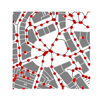
Along the skeleton of the urban open space

The aim here is to use the virtual sensor positioning strategy presented in (Rodler & Leduc, 2019). The first step is therefore to determine the skeleton of the open space using the following geoprocessing:

STSkeletonizeTheVoid(gdf, samplingDist=10.0)

The constructor of this class has two arguments. The first is the GeoDataFrame of the building footprints and the second is the sampling distance between two consecutive points located on the building contours. These points are used in the tessellation process. Once the skeleton of the open space is obtained, it only remains to sample it in a set of points with the previously mentioned geoprocessing:

STPointsDensifier(gdf, distance, pathidFieldname=None, adjustableDist=True, removeDuplicate=True)

The following code snippet summarizes the entire process:

from t4gpd.demos.GeoDataFrameDemos import GeoDataFrameDemos
from t4gpd.morph.STPointsDensifier import STPointsDensifier
from t4gpd.morph.STSkeletonizeTheVoid import STSkeletonizeTheVoid

buildings = GeoDataFrameDemos.districtRoyaleInNantesBuildings()

skeleton = STSkeletonizeTheVoid(buildings, samplingDist=5.0).run()

sensors = STPointsDensifier(skeleton, distance=15.0, 
    adjustableDist=True, removeDuplicate=False).run()

To map it via matplotlib, proceed as follows:

import matplotlib.pyplot as plt
from shapely.geometry import box

minx, miny, maxx, maxy = box(*buildings.total_bounds).buffer(-70).bounds

_, basemap = plt.subplots(figsize=(0.25*8.26, 0.25*8.26))
buildings.plot(ax=basemap, color='grey', edgecolor='white', linewidth=0.5)
skeleton.plot(ax=basemap, color='black', linewidth=0.5)
sensors.plot(ax=basemap, color='red', marker='.')

basemap.axis([minx, maxx, miny, maxy])
plt.axis('off')
plt.savefig('img/demo6.png')

Meshing of the urban space

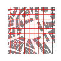
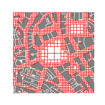
Grid the region of interest

Gridding is a well-known spatial sampling technique. To grid a study space, t4gpd provides the geoprocessing name t4gpd.morph.STGrid.

STGrid(gdf, dx, dy=None, indoor=None, intoPoint=False, encode=True)

If you want to grid the region of interest proceed as follows:

from t4gpd.demos.GeoDataFrameDemos import GeoDataFrameDemos
from t4gpd.morph.STGrid import STGrid

buildings = GeoDataFrameDemos.districtRoyaleInNantesBuildings()

grid = STGrid(buildings, dx=20, dy=None, indoor=None, intoPoint=False).run()

To map the resulting grid via matplotlib, proceed as follows:

import matplotlib.pyplot as plt
from shapely.geometry import box

minx, miny, maxx, maxy = box(*buildings.total_bounds).buffer(-50).bounds

_, basemap = plt.subplots(figsize=(0.25*8.26, 0.25*8.26))
buildings.plot(ax=basemap, color='grey', edgecolor='white', linewidth=0.5)
grid.boundary.plot(ax=basemap, color='red', linewidth=0.5)

basemap.axis([minx, maxx, miny, maxy])
plt.axis('off')
plt.savefig('img/demo7.png')

Adaptive meshing of a region of interest

Adaptive gridding is a well-known spatial sampling technique. To adaptively grid a study space, t4gpd provides the geoprocessing name t4gpd.morph.STAdaptativeGrid.

STAdaptativeGrid(gdf, dx, thresholds=None, indoor=False, intoPoint=False, encode=True)

If you want to adaptively grid the region of interest proceed as follows:

from t4gpd.demos.GeoDataFrameDemos import GeoDataFrameDemos
from t4gpd.morph.STAdaptativeGrid import STAdaptativeGrid

buildings = GeoDataFrameDemos.districtRoyaleInNantesBuildings()

grid = STAdaptativeGrid(buildings, dx=[32, 16, 8, 4], indoor=False, intoPoint=False).run()

To map the resulting grid via matplotlib, proceed as follows:

import matplotlib.pyplot as plt
from shapely.geometry import box

minx, miny, maxx, maxy = box(*buildings.total_bounds).buffer(-50).bounds

_, basemap = plt.subplots(figsize=(0.25*8.26, 0.25*8.26))
buildings.plot(ax=basemap, color='grey', edgecolor='white', linewidth=0.5)
grid.boundary.plot(ax=basemap, color='red', linewidth=0.5)

basemap.axis([minx, maxx, miny, maxy])
plt.axis('off')
plt.savefig('img/demo8.png')

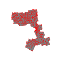
How to build a Triangulated irregular network (TIN)

The mesh we will produce here assumes that you have installed the GMSH three-dimensional finite element mesh generator. The class t4gpd.morph.GmshTriangulator is a wrapper that encapsulates an export to GMSH/Geo format, a call to the GMSH mesher and an import of the GMSH/MSH file format result.

GmshTriangulator(gdf, characteristicLength=10.0, gmsh=None)

As you can see from the following code snippet, the gmsh argument of the GmshTriangulator command is used to specify the location of the GMSH executable.

from t4gpd.demos.GeoDataFrameDemos import GeoDataFrameDemos
from t4gpd.morph.GmshTriangulator import GmshTriangulator

building = GeoDataFrameDemos.singleBuildingInNantes()
tin = GmshTriangulator(building, characteristicLength=15.0,
    gmsh='/usr/bin/gmsh').run()

To map the resulting mesh via matplotlib, proceed as follows:

import matplotlib.pyplot as plt

_, basemap = plt.subplots(figsize=(0.25*8.26, 0.25*8.26))
building.plot(ax=basemap, color='grey', edgecolor='white', linewidth=0.5)
tin.boundary.plot(ax=basemap, color='red', linewidth=0.25)

plt.axis('off')
plt.savefig('img/demo9.png')

How to snap points on line?

There are two distinct possibilities, either via the t4gpd.morph.STSnappingPointsOnLines class, or via the t4gpd.morph.STSnappingPointsOnLines2 class.