Urban morphometry

Generation of enclosing shapes

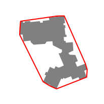
Convex Hull

The t4gpd class named ConvexHull is a wrapper for the Shapely convex_hull method. To use it, an instance of ConvexHull must be passed as the first argument of the STGeoProcess constructor as in the following example. The resulting red object is a GeoPandas GeoDataFrame.

from t4gpd.demos.GeoDataFrameDemos import GeoDataFrameDemos
from t4gpd.morph.geoProcesses.ConvexHull import ConvexHull
from t4gpd.morph.geoProcesses.STGeoProcess import STGeoProcess

building = GeoDataFrameDemos.singleBuildingInNantes()
red = STGeoProcess(ConvexHull(), building).run()

The following code snippet allows to map these two GeoDataFrame.

import matplotlib.pyplot as plt
_, basemap = plt.subplots(figsize=(0.25*8.26, 0.25*8.26))
building.plot(ax=basemap, color='grey')
red.boundary.plot(ax=basemap, color='red')
plt.axis('off')
plt.savefig('img/convex_hull.png')

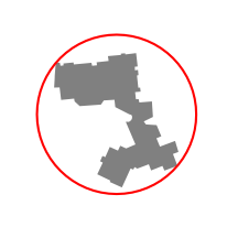
Minimum Bounding Circle

To determine the Minimum-area Bounding Circle, we implemented the Chrystal Algorithm. The t4gpd class with the name MBC allows, as before, when it is passed as the first argument of the STGeoProcess constructor to implement the corresponding mechanism.

from t4gpd.demos.GeoDataFrameDemos import GeoDataFrameDemos
from t4gpd.morph.geoProcesses.MBC import MBC
from t4gpd.morph.geoProcesses.STGeoProcess import STGeoProcess

building = GeoDataFrameDemos.singleBuildingInNantes()
red = STGeoProcess(MBC(), building).run()

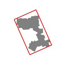
Minimum-area Bounding Rectangle

To determine the Minimum-area Bounding Rectangle, we wrapped the shapely method named minimum_rotated_rectangle. To activate it, the MABR class must be passed as the first argument of the STGeoProcess constructor.

from t4gpd.demos.GeoDataFrameDemos import GeoDataFrameDemos
from t4gpd.morph.geoProcesses.MABR import MABR
from t4gpd.morph.geoProcesses.STGeoProcess import STGeoProcess

building = GeoDataFrameDemos.singleBuildingInNantes()
red = STGeoProcess(MABR(), building).run()

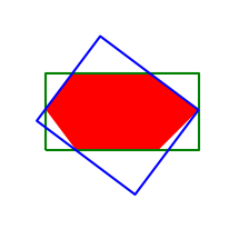
Note: Substituting the MPBR class name to the MABR one, allows to recover the Minimum-Perimeter Bounding Rectangle. As can be seen from the following example taken from (Leduc & Leduc, 2020), MABR and MPBR can be quite different.

import matplotlib.pyplot as plt
from geopandas import GeoDataFrame
from shapely.wkt import loads
from t4gpd.morph.geoProcesses.MABR import MABR
from t4gpd.morph.geoProcesses.MPBR import MPBR
from t4gpd.morph.geoProcesses.STGeoProcess import STGeoProcess

red = GeoDataFrame([{'geometry': 
    loads('POLYGON ((1 1, 3 1, 4 2, 2.8 2.9, 0.9 2.9, 0.25 2, 1 1))')}])
green = STGeoProcess(MABR(), red).run()
blue = STGeoProcess(MPBR(), red).run()

_, basemap = plt.subplots(figsize=(0.25*8.26, 0.25*8.26))
red.plot(ax=basemap, color='red')
green.boundary.plot(ax=basemap, color='green')
blue.boundary.plot(ax=basemap, color='blue')
plt.axis('off')
plt.savefig('img/mabr_vs_mpbr.png')

Indeed, the green MABR has an area of 7.125 m² and a perimeter of 11.3 m, while the blue MPBR has an area of 7.852 m² and a perimeter of 11.24 m.

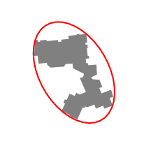
Minimum-Area Bounding Ellipse

To determine the Minimum-Area Bounding Ellipse, we used the algorithm presented in (Leduc & Leduc, 2020). To activate it, a MABE instance must be passed as the first argument of the STGeoProcess constructor. The threshold argument is an angular value in radians. It is used to prune the almost flat angles of the given geometries.

MABE(npoints=40, threshold=None)

from t4gpd.demos.GeoDataFrameDemos import GeoDataFrameDemos
from t4gpd.morph.geoProcesses.MABE import MABE
from t4gpd.morph.geoProcesses.STGeoProcess import STGeoProcess

building = GeoDataFrameDemos.singleBuildingInNantes()
red = STGeoProcess(MABE(npoints=40, threshold=None), building).run()

Convexity indices

There are various convexity indices among which we have implemented:

• The number of convex components. This dimensionless indicator corresponds to the number of concavities in the shape. In the resulting GeoDataFrame, the corresponding column is named n_con_comp.

• The surface convexity defect. This indicator is dimensionless and standardized. It is equal to the ratio of the area of the shape to that of its convex hull. In the resulting GeoDataFrame, the corresponding column is named a_conv_def.

• The perimeter convexity defect. In the resulting GeoDataFrame, the corresponding column is named p_conv_def.

from t4gpd.demos.GeoDataFrameDemos import GeoDataFrameDemos
from t4gpd.morph.geoProcesses.ConvexityIndices import ConvexityIndices
from t4gpd.morph.geoProcesses.STGeoProcess import STGeoProcess

building = GeoDataFrameDemos.singleBuildingInNantes()

result = STGeoProcess(ConvexityIndices, building).run()
result = result[['n_con_comp', 'a_conv_def', 'p_conv_def', 'big_concav', 'small_conc']]
print(result) # 8, 58.9%, 65.0%, 152838.8, 6.0

Circularity indices

from t4gpd.demos.GeoDataFrameDemos import GeoDataFrameDemos
from t4gpd.morph.geoProcesses.CircularityIndices import CircularityIndices
from t4gpd.morph.geoProcesses.STGeoProcess import STGeoProcess

building = GeoDataFrameDemos.singleBuildingInNantes()

result = STGeoProcess(CircularityIndices, building).run()
result = result[['gravelius', 'jaggedness', 'miller', 'morton', 'a_circ_def']]
print(result) # 2.2, 61.5, 20.4%, 32.7%, 32.7%

Rectangularity indices

from t4gpd.demos.GeoDataFrameDemos import GeoDataFrameDemos
from t4gpd.morph.geoProcesses.RectangularityIndices import RectangularityIndices
from t4gpd.morph.geoProcesses.STGeoProcess import STGeoProcess

building = GeoDataFrameDemos.singleBuildingInNantes()

result = STGeoProcess(RectangularityIndices, building).run()
result = result[['stretching', 'a_rect_def', 'p_rect_def']]
print(result) # 62.0%, 51.2%, 73.3%

Ellipticity indices

from t4gpd.demos.GeoDataFrameDemos import GeoDataFrameDemos
from t4gpd.morph.geoProcesses.EllipticityIndices import EllipticityIndices
from t4gpd.morph.geoProcesses.STGeoProcess import STGeoProcess

building = GeoDataFrameDemos.singleBuildingInNantes()

result = STGeoProcess(EllipticityIndices(threshold=None), building).run()
result = result[['flattening', 'a_elli_def', 'p_elli_def']]
print(result) # 62.9%, 44.3%, 70.6%