Urban bioclimatic shape analysis

Sky View Factor

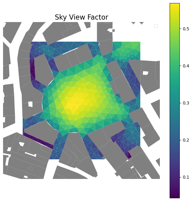
The sky view factor is a synthetic indicator that aims to quantify, at any point in the urban environment, the openness of space and, more specifically, the potential to see the sky. This indicator varies from 0 (the sky is absolutely not visible) to 1 (the view of the sky is not hindered by any mask). This indicator and its implementation are more precisely described in (Rodler and Leduc, 2019).

In the following example, we first mesh the space (via the t4gpd.morph.GmshTriangulator) and then calculate the SVF in the centroid of each mesh. For this purpose, we use the class t4gpd.morph.geoProcesses.SkyViewFactor.

import geopandas as gpd, matplotlib.pyplot as plt
from shapely.geometry import box, Point
from t4gpd.demos.GeoDataFrameDemos import GeoDataFrameDemos
from t4gpd.morph.GmshTriangulator import GmshTriangulator
from t4gpd.morph.STExtractOpenSpaces import STExtractOpenSpaces
from t4gpd.morph.geoProcesses.STGeoProcess import STGeoProcess
from t4gpd.morph.geoProcesses.SkyViewFactor import SkyViewFactor

buildings = GeoDataFrameDemos.districtRoyaleInNantesBuildings()

roi = box(*Point((355187.0, 6689306.0)).buffer(60.0).bounds)
roi = gpd.GeoDataFrame([{'geometry': roi}], crs=buildings.crs)

void = STExtractOpenSpaces(roi, buildings).run()
void = void.explode()
void = void[void.area > 100]
void.geometry = void.simplify(tolerance=1.0, preserve_topology=True)
sensors = GmshTriangulator(void, characteristicLength=10.0, 
    gmsh = '/usr/local/bin/gmsh').run()

op = SkyViewFactor(buildings, nRays=64, maxRayLen=100.0,
    elevationFieldname='HAUTEUR', method=2018, background=True)
sensors = STGeoProcess(op, sensors).run()

minx, miny, maxx, maxy = roi.buffer(20.0).total_bounds

_, basemap = plt.subplots(figsize=(8.26, 8.26))
basemap.set_title('Sky View Factor', fontsize=16)
plt.axis('off')
buildings.plot(ax=basemap, color='grey')
sensors.plot(ax=basemap, column='svf', markersize=8, 
    legend=True, cmap='viridis')
plt.axis([minx, maxx, miny, maxy])
plt.legend(loc = 'upper right', framealpha=0.5)
plt.savefig('img/svf.png', bbox_inches='tight')

Ground shadows

Some of the following features are implemented in (Leduc et al., 2021).

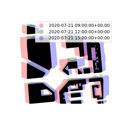
Ground shadows of buildings

The aim here is to determine the ground shadows of buildings assimilated to a collection of straight prisms. To do this, the GeoDataFrame of the building footprints (polygonal footprints completed with a height attribute name) and a set of dates are provided to the t4gpd.sun.STHardShadow class. This double information makes it possible to determine the layout of the shadows of the buildings, the latitude being recovered from the centroid of the zone of the buildings.

STHardShadow(occludersGdf, datetimes, occludersElevationFieldname='HAUTEUR', altitudeOfShadowPlane=0, aggregate=False, tz=None, model='pysolar')

from datetime import datetime, timedelta
from t4gpd.commons.DatetimeLib import DatetimeLib
from t4gpd.demos.GeoDataFrameDemos import GeoDataFrameDemos
from t4gpd.sun.STHardShadow import STHardShadow

buildings = GeoDataFrameDemos.ensaNantesBuildings()

datetimes = [datetime(2020, 7, 21, 9), datetime(2020, 7, 21, 15), timedelta(hours=3)]
datetimes = DatetimeLib.generate(datetimes)
shadows = STHardShadow(buildings, datetimes, occludersElevationFieldname='HAUTEUR',
    altitudeOfShadowPlane=0, aggregate=True, tz=None, model='pysolar').run()

To map it via matplotlib, proceed as follows:

import matplotlib.pyplot as plt
from matplotlib.colors import ListedColormap

my_cmap = ListedColormap(['red', 'green', 'blue'])

_, basemap = plt.subplots(figsize=(0.5 * 8.26, 0.5 * 8.26))
shadows.plot(ax=basemap, column='datetime', cmap=my_cmap, alpha=0.3, legend=True)
buildings.plot(ax=basemap, color='black')
plt.axis('off')
plt.savefig('img/shadows1.png')

Tree shadows

In order to plot the ground shadows caused by trees, we implemented two distinct tree models. The first one is a model for which the tree crown is spherical. It corresponds to the class t4gpd.sun.STTreeHardShadow. The second is a model for which the tree crown is a conical frustum (i.e. possibly a cyclinder). It corresponds to the class t4gpd.sun.STTreeHardShadow2.

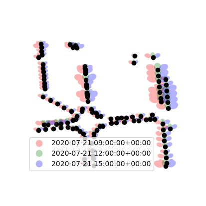
Shadows cast by trees with spherical crowns

Ground shadows caused by trees with spherical crowns are ellipses. The t4gpd.sun.STTreeHardShadow class is used to draw their contours.

STTreeHardShadow(treesGdf, datetimes, treeHeightFieldname, treeCrownRadiusFieldname, altitudeOfShadowPlane=0, aggregate=False, tz=None, model='pysolar', npoints=32)

We start here by establishing an arbitrary correspondence map, named TREES, between the height estimate (an interval stored as a string) and the total height on the one hand and the radius of the cylindrical crown on the other hand.

from datetime import datetime, timedelta
from t4gpd.commons.DatetimeLib import DatetimeLib
from t4gpd.demos.GeoDataFrameDemos import GeoDataFrameDemos
from t4gpd.sun.STTreeHardShadow import STTreeHardShadow

TREES = {
    '0-5 m':   {'height': 5.0,  'radius': 2.0},
    '6-10 m':  {'height': 8.0,  'radius': 3.0},
    '11-15 m': {'height': 13.0, 'radius': 4.0},
    '16-20 m': {'height': 18.0, 'radius': 6.0},
    'Z.N.R':   {'height': 10.0, 'radius': 3.0},
    '21-30 m': {'height': 25.5, 'radius': 8.0}
}

trees = GeoDataFrameDemos.ensaNantesTrees()
trees['height'] = trees.hauteur.apply(lambda h: TREES[h]['height'])
trees['radius'] = trees.hauteur.apply(lambda h: TREES[h]['radius'])

datetimes = [datetime(2020, 7, 21, 9), datetime(2020, 7, 21, 15), timedelta(hours=3)]
datetimes = DatetimeLib.generate(datetimes)
shadows = STTreeHardShadow(trees, datetimes, treeHeightFieldname='height',
    treeCrownRadiusFieldname='radius',  altitudeOfShadowPlane=0, 
    aggregate=True, tz=None, model='pysolar', npoints=32).run()

To map it via matplotlib, proceed as follows:

import matplotlib.pyplot as plt
from matplotlib.colors import ListedColormap

my_cmap = ListedColormap(['red', 'green', 'blue'])

_, basemap = plt.subplots(figsize=(0.5 * 8.26, 0.5 * 8.26))
shadows.plot(ax=basemap, column='datetime', cmap=my_cmap, alpha=0.3, legend=True)
trees.plot(ax=basemap, color='black')
plt.axis('off')
plt.savefig('img/shadows2.png')

Shadows cast by trees with conical frustum-like crowns

STTreeHardShadow2(treesGdf, datetimes, treeHeightFieldname, treeCrownHeightFieldname, treeUpperCrownRadiusFieldname, treeLowerCrownRadiusFieldname, altitudeOfShadowPlane=0, aggregate=False, tz=None, model='pysolar', npoints=32)

We start here by establishing an arbitrary correspondence map, named TREES, between the height estimate (an interval stored as a string) and the total height on the one hand and the radius of the cylindrical crown on the other hand.

from datetime import datetime, timedelta
from t4gpd.commons.DatetimeLib import DatetimeLib
from t4gpd.demos.GeoDataFrameDemos import GeoDataFrameDemos
from t4gpd.sun.STTreeHardShadow2 import STTreeHardShadow2

TREES = {
    '0-5 m':   {'height': 5.0,  'crown_height': 2.0,  'radius': 2.0},
    '6-10 m':  {'height': 8.0,  'crown_height': 5.0,  'radius': 3.0},
    '11-15 m': {'height': 13.0, 'crown_height': 9.0,  'radius': 4.0},
    '16-20 m': {'height': 18.0, 'crown_height': 14.0, 'radius': 6.0},
    'Z.N.R':   {'height': 10.0, 'crown_height': 6.0,  'radius': 3.0},
    '21-30 m': {'height': 25.5, 'crown_height': 21.0, 'radius': 8.0}
}

trees = GeoDataFrameDemos.ensaNantesTrees()
trees['height'] = trees.hauteur.apply(lambda h: TREES[h]['height'])
trees['crown_height'] = trees.hauteur.apply(lambda h: TREES[h]['crown_height'])
trees['crown_radiusL'] = trees.hauteur.apply(lambda h: TREES[h]['radius'])
trees['crown_radiusU'] = trees.hauteur.apply(lambda h: TREES[h]['radius']-1.5)

datetimes = [datetime(2020, 7, 21, 9), datetime(2020, 7, 21, 15), timedelta(hours=3)]
datetimes = DatetimeLib.generate(datetimes)
shadows = STTreeHardShadow2(trees, datetimes, treeHeightFieldname='height',
    treeCrownHeightFieldname='crown_height',
    treeUpperCrownRadiusFieldname='crown_radiusU', 
    treeLowerCrownRadiusFieldname='crown_radiusL',
    altitudeOfShadowPlane=0, aggregate=False, tz=None, model='pysolar', npoints=32).run()

To map it via matplotlib, proceed as follows:

import matplotlib.pyplot as plt
from matplotlib.colors import ListedColormap

my_cmap = ListedColormap(['red', 'green', 'blue'])

_, basemap = plt.subplots(figsize=(0.5 * 8.26, 0.5 * 8.26))
shadows.plot(ax=basemap, column='datetime', cmap=my_cmap, alpha=0.3, legend=True)
trees.plot(ax=basemap, color='black')
plt.axis('off')
plt.savefig('img/shadows3.png')