Urban landscape analysis

Isovist and isovist field

In 2D, the set of points on the map plane that are directly visible from the point of view (also called the generation point) is called isovist. In the case where no opaque surface stops the field of view, it is sometimes necessary to impose an artificial horizon to limit the range.

To analyze space in a more systematic way over a territory, Benedikt (1979) proposes the notion of isovist field. This is an extrapolation of the mathematical notion of scalar field (resp. vector field) which associates a scalar (resp. a vector) with any point in Euclidean space. If the isovist describes the space surrounding a given point, the isovist field associates, to any point of the study area, an isovist. The isovist field thus gives access to the description property of the enveloping space at any point of interest.

STIsovistField2D(buildings, viewpoints, nRays=64, rayLength=100.0)

from geopandas import GeoDataFrame
from shapely.geometry import Point
from t4gpd.demos.GeoDataFrameDemos import GeoDataFrameDemos
from t4gpd.isovist.STIsovistField2D import STIsovistField2D

buildings = GeoDataFrameDemos.districtRoyaleInNantesBuildings()

pts = [ Point((355143.0, 6689359.4)), Point((355151.5, 6689310.1)) ]
viewpoints = GeoDataFrame([{'gid': i, 'geometry': p} for i,p in enumerate(pts)],
    crs=buildings.crs)

isovRays, isovists = STIsovistField2D(buildings, viewpoints, nRays=180, rayLength=200.0).run()

To map it via matplotlib, proceed as follows:

import matplotlib.pyplot as plt
from shapely.geometry import box

_, basemap = plt.subplots(figsize=(0.5*8.26, 0.5*8.26))
buildings.plot(ax=basemap, color='lightgrey', edgecolor='white', linewidth=0.5)
isovists.plot(ax=basemap, edgecolor='dimgrey', color='yellow', alpha=0.85)
viewpoints.plot(ax=basemap, color='black', marker='+')
plt.axis('off')
plt.savefig('img/isovists.png')

Indices for star-shaped polygons

An isovist is, by nature, star-shaped. As noted by Piombini et al. (2014), because of this topological property, such a shape can be described by simply transcribing its contour into a radial distance function. This radial distance function associates to a given azimuth (from the angular abscissa discretization) the length of the radius connecting the viewpoint to the corresponding contour point. Most of the shape indices presented below analyze this radial distance function as a simple distribution of a real variable.

Some of these shape indices are implemented in the class t4gpd.morph.geoProcesses.StarShapedIndices. Using this class helps quantify - for each tuple of the already defined GeoDataFrame isovRays - the eccentricity (drift), the minimum length (resp. average, maximum or standard deviation) of the rays, or the entropy of the radial distance function.

from t4gpd.morph.geoProcesses.STGeoProcess import STGeoProcess
from t4gpd.morph.geoProcesses.StarShapedIndices import StarShapedIndices

result = STGeoProcess(StarShapedIndices(precision=1.0, base=2), isovRays).run()

print(result[['gid', 'drift', 'min_raylen', 'avg_raylen', 
              'std_raylen', 'max_raylen', 'entropy']])

Sky Map

SkyMap2D(gdf, nRays=180, size=4.0, maxRayLen=100.0, elevationFieldname='HAUTEUR', projectionName='Stereographic')

from geopandas import GeoDataFrame
from shapely.geometry import Point
from t4gpd.demos.GeoDataFrameDemos import GeoDataFrameDemos
from t4gpd.morph.geoProcesses.SkyMap2D import SkyMap2D
from t4gpd.morph.geoProcesses.STGeoProcess import STGeoProcess

buildings = GeoDataFrameDemos.districtRoyaleInNantesBuildings()

pts = [ Point((355154.0, 6689292.4)), Point((355206.0, 6689346.6)),
    Point((355229.6, 6689294.1)), Point((355190.5, 6689306.1)),
    Point((355143.0, 6689359.4)) ]
viewpoints = GeoDataFrame([{'geometry': p} for p in pts], crs=buildings.crs)

op = SkyMap2D(buildings, nRays=180, size=8.0, maxRayLen=100.0, 
    elevationFieldname='HAUTEUR', projectionName='Stereographic')
skymaps = STGeoProcess(op, viewpoints).run()

To map it via matplotlib, proceed as follows:

import matplotlib.pyplot as plt
from shapely.geometry import box

minx, miny, maxx, maxy = box(*skymaps.total_bounds).buffer(10).bounds

_, basemap = plt.subplots(figsize=(0.75*8.26, 0.75*8.26))
buildings.plot(ax=basemap, color='lightgrey', edgecolor='white', linewidth=0.5)
skymaps.plot(ax=basemap, color='dimgrey')
viewpoints.plot(ax=basemap, color='black', marker='+')
plt.axis('off')
plt.axis([minx, maxx, miny, maxy])
plt.savefig('img/skymaps.png')

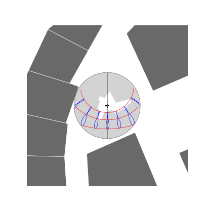
Sky and Sun Maps

SkyMap2D(gdf, nRays=180, size=4.0, maxRayLen=100.0, elevationFieldname='HAUTEUR', projectionName='Stereographic')

STSunMap2D(viewpointsGdf, datetimes, size=4.0, projectionName='Stereographic', tz=None, model='pysolar')

from datetime import date, time
from geopandas import GeoDataFrame
from shapely.geometry import Point
from t4gpd.demos.GeoDataFrameDemos import GeoDataFrameDemos
from t4gpd.morph.geoProcesses.SkyMap2D import SkyMap2D
from t4gpd.morph.geoProcesses.STGeoProcess import STGeoProcess
from t4gpd.sun.STSunMap2D import STSunMap2D

buildings = GeoDataFrameDemos.districtRoyaleInNantesBuildings()
viewpoint = GeoDataFrame([{'geometry': Point((355143.0, 6689359.4))}],
    crs=buildings.crs)

op = SkyMap2D(buildings, nRays=180, size=7.0, maxRayLen=100.0, 
    elevationFieldname='HAUTEUR', projectionName='Stereographic')
skymap = STGeoProcess(op, viewpoint).run()

datetimes = [ date(2020, month, 21) for month in (3, 6, 12)]
datetimes += [ time(hour) for hour in range(6, 19, 2) ]

sunmap = STSunMap2D(viewpoint, datetimes, size=7.0,
    projectionName='Stereographic').run()

To map it via matplotlib, proceed as follows:

import matplotlib.pyplot as plt
from shapely.geometry import box

minx, miny, maxx, maxy = box(*skymap.total_bounds).buffer(10).bounds

_, basemap = plt.subplots(figsize=(0.5*8.26, 0.5*8.26))
buildings.plot(ax=basemap, color='dimgrey', edgecolor='white', linewidth=0.5)

skymap.plot(ax=basemap, color='lightgrey')
viewpoint.plot(ax=basemap, color='black', marker='+')
sunmap[ sunmap.label == 'framework' ].plot(ax=basemap, linewidth=0.5, color='dimgrey')
sunmap[ sunmap.label.str.startswith('2020-') ].plot(ax=basemap, linewidth=0.5, color='red')
sunmap[ sunmap.label.str.endswith(':00:00') ].plot(ax=basemap, linewidth=0.5, color='blue')
plt.axis('off')
plt.axis([minx, maxx, miny, maxy])
plt.savefig('img/skySunMaps.png')